Neurons vs Perceptrons
Artificial neurons simplify the brain by swapping out messy, time-dependent chemistry for clean, instantaneous arithmetic.
Dieser Inhalt ist noch nicht in deiner Sprache verfügbar.
Biological Neurons
Section titled “Biological Neurons”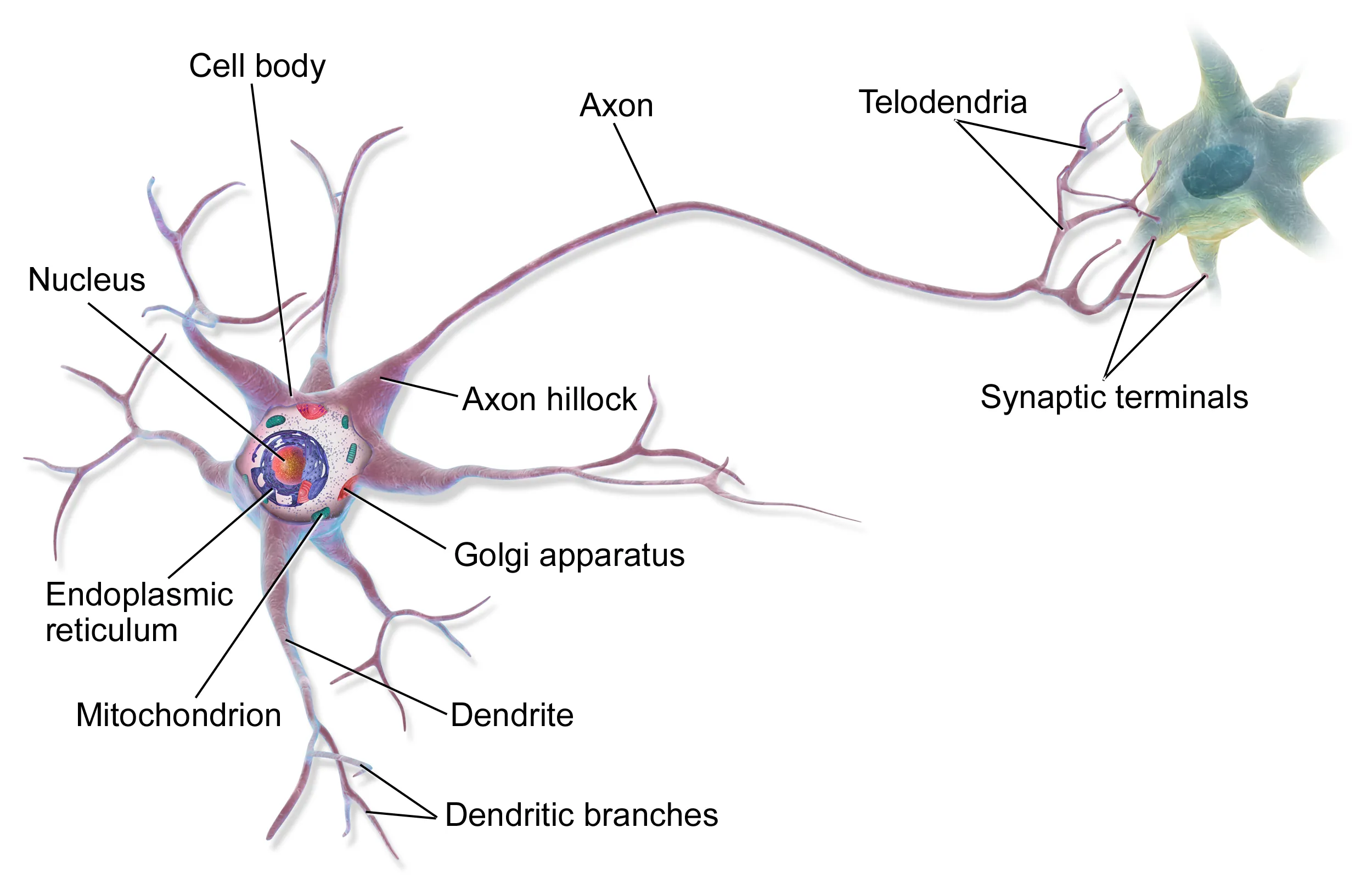

Artificial Neurons
Section titled “Artificial Neurons”An artificial neuron (often called a perceptron or node) reduces the biological anatomy into a single mathematical function. Artificial neural networks (ANNs) are mathematical abstractions rather than perfect biological replicas to make them computationally feasible:
1. Structural Simplification
Section titled “1. Structural Simplification”- Dendrites $\rightarrow$ Inputs: Biological dendrites receive complex electrochemical signals from thousands of neighboring cells. In an artificial neuron, these are simplified into a static vector of numerical inputs.
- Synapses $\rightarrow$ Weights: Synaptic plasticity is simplified into static numbers called weights. Multiplying the input by the weight simulates the strengthening or weakening of a signal.
- Soma $\rightarrow$ Summation: The soma biologically sums up electrical potential changes. The artificial neuron simplifies this into a basic linear algebra operation: a weighted sum plus a baseline offset called a bias.
- Axon $\rightarrow$ Output: The biological axon transmits the final signal to the next neuron. In code, this is simply the final numerical output of the function passed along a data pipeline.
2. Functional & Signal Simplification
Section titled “2. Functional & Signal Simplification”- Electrochemical Spikes –> Static Numbers: Continuous-time electrical pulses (action potentials) and chemical neurotransmitters vs. discrete floating-point values.
- Asynchronous & Time-Dependent –> Synchronous: Signals depend heavily on when they arrive (temporal summation) vs calculations happen instantly and simultaneously in rigid mathematical passes (forward propagation).
- All-or-Nothing –> Continuous/Graded: A biological neuron either fires a full spike or doesn’t fire at all based on a strict voltage threshold vs. continuous mathematical activation functions (like ReLU, Sigmoid, or Tanh) that output smooth, fractional values instead of binary spikes.
3. The Learning Simplification (Backpropagation)
Section titled “3. The Learning Simplification (Backpropagation)”Perhaps the biggest deviation from biology is how these neurons learn:
- Biological Learning: In the brain, learning is largely local and self-organizing (often summarized by Hebbian theory: “neurons that fire together, wire together”). A neuron adjusts its connections based on the activity of its immediate neighbors.
- Artificial Learning: ANNs rely on a global optimization algorithm called Backpropagation. It requires a centralized “loss function” to calculate an error rate, which is then sent backward through the entire network using calculus (the chain rule) to adjust every weight perfectly. The biological brain cannot calculate global gradients in this manner.
Summary: An artificial neuron simplifies the brain by swapping out messy, time-dependent chemistry for clean, instantaneous arithmetic. It replaces the binary, electrochemical “spike” of a real brain cell with a simple weighted sum passed through a continuous mathematical function.
Conclusion: While a more complex model of an artificial neuron is possible, without specialized hardware, it isn’t efficient or scalable. The connectionist paradigm’s simple arithmetic aligns well with the currently available hardware (GPUs and TPUs) allowing for the large, even massive, models.